Über die letzten Wochen habe ich an einer App zur automatischen Ermittlung, Visualisierung und Korrektur von Publikationsbias in Meta-Analysen gearbeitet und denke, dass ich es bei der jetzigen (zufriedenstellenden) Version belassen werde. Das Programm beginnt mit dem Input der Daten der kontrollierten Experimente (RCTs). Diese können direkt aus der Meta-Studie entnommen werden. Da Meta-Studien die RCT-Daten oft unterschiedlich präsentieren, habe ich vier Modi zum Input bereitgestellt. Wenn die Meta-Studie die Effektstärken und Grenzen der jeweiligen 95 % Konfidenzintervalle berichtet, bieten sich die ersten beiden Input-Modi an:
- Input-Modus 1: Input als drei separate Listen. Liste der Effektstärken d = [0.30, 0.42, 0.08], Liste der unteren Grenzen dlow = [-0.20, 0.04, -0.48], Liste der oberen Grenzen dhigh = [0.50, 0.80, 0.54].
- Input-Modus 2: Input als eine Liste der Abfolge d, dlow, dhigh. Zum Beispiel: l = [0.30, -0.20, 0.50, 0.42, 0.04, 0.80, 0.08, -0.48, 0.54].
Sind statt der Grenzen die Standardfehler oder Varianzen gegeben, was ziemlich oft der Fall ist, kann man die anderen beiden anderen Input-Modi nutzen. Die Grenzen des 95 % KI werden dann automatisch vor der Analyse berechnet.
- Input-Modus 3: Input als eine Liste der Abfolge d, SE. Zum Beispiel: lse = [0.30, 0.18, 0.42, 0.25, 0.08, 0.24]
- Input-Modus 3: Input als eine Liste der Abfolge d, Var. Zum Beispiel: lv = [0.30, 0.03, 0.42, 0.05, 0.08, 0.04]
Eine bestimmte Reihenfolge muss dabei nicht eingehalten werden. Notwendige Sortierungen werden automatisch gemacht. Da ein Teil der Ermittlung und Korrektur des Publikationsbias darauf basiert, eine Neuberechnung der Meta-Analyse mit Beschränkung auf die Top k RCTs vorzunehmen, muss dieser Wert k als Input gegeben werden. Top k RCTs meint hier die Anzahl k RCTs mit dem geringsten Standardfehler (höchste Probantenzahlen).
Mit der Variable fixed_mode = 1 lässt sich eine Meta-Analyse nach dem Fixed-Effects-Model erzwingen. Standardmäßig ist fixed_mode = 0 und es erfolgt eine Analyse nach dem Random-Effects-Model. Ein letzter möglicher Input ist die Aktivierung des Comparison Mode, darauf gehe ich aber später ein.
Zuerst rechnet das Programm die gesamte Meta-Analyse nach, beginnend mit der Berechnung von Cochrane’s Q, der Heterogenität I² und der Zwischen-Studien-Varianz Tau² sowie einem Histogramm der Effektstärken.

Danach werden Charakteristiken der einzelnen RCTs berechnet und angezeigt. Dazu gehören die Gewichte, mit denen die jeweiligen RCTs in die Meta-Analyse einfließen, sowie die jeweiligen Probantenzahlen, mittlere Probantenzahl pro RCT und gesamte Probantenzahl der RCTs. Das gefolgt von einem Histogramm der Probantenzahlen.

Zum Schluss die Meta-Analyse (nach Borenstein) und die Resultate: Varianz des Effekts, Standardfehler des Effekts, Effektstärke inklusive 95 % Konfidenzintervall, p-Wert der Differenz zum Nulleffekt und H0C als Maß für die Sicherheit der Ablehnung der Nullhypothese.

Dann beginnt der eigentliche Job: Publikationsbias ermitteln und wenn nötig korrigieren. Teil I basiert auf dem Prinzip der Konvergenz zum wahren Effekt. Man nimmt an, dass je größer die Studie, desto näher liegt der gefundene Effekt am wahren Effekt. Die Meta-Analyse wird also nochmals berechnet mit Beschränkung auf die k RCTs mit dem geringsten Standardfehler. Das Programm sortiert die Inputs, kürzt sie und berechnet die Gewichte neu. Tau² und der Standardfehler des Effekts wird explizit nicht neu berechnet. Das hat sehr gute Gründe (siehe Anmerkungen).
Das Programm zeigt dann das Resultat im gleichen Format an und wertet die Differenz zur kompletten Meta-Analyse. Es wird angenommen, dass jegliche Verschiebung der Effektstärke infolge des Publikationsbias geschieht. Es wird gewertet, ob der Einfluss des Publikationsbias auf die Effektstärke signifikant ist (und bei welchem p-Niveau) und ob die Effekt-Verschiebung die Sicherheit bei der Ablehnung der Nullhypothese maßgeblich berührt. Danch wird noch ein Plot der Unterschiede generiert. Für die Analyse des Funnel Plots in Teil II des Programms wird angenommen, dass die hier gefundene Effektstärke die wahre Effektstärke ist.

In Teil II wird versucht, Asymmetrien des Funnel Plots zu quantifizieren und somit eine ergänzende Einschätzung zum Publikationsbias zu liefern. Alle Effekstärken werden zuerst auf die in Teil I gefundene Effektstärke zentriert. Dann wird der Plot der Effekte oberhalb 0 gemacht, die Regressionsgerade berechnet, der Plot der Effekte unterhalb 0 generiert, wieder die Regressionsgerade berechnet und schlussendlich der gesamte Funnel Plot inklusive der Geraden gezeigt.


Jetzt werden die Asymmetrien berechnet:
- Asymmetrie der Steigung der Geraden
- Asymmetrie der Anzahl RCTs
- Asymmetrie der Anzahl Ausreißer
- Asymmetrie der Summe der Distanzen zur Mittellinie
- Asymmetrie der maximalen Abweichungen zur Mittellinie
Zu jeder Asymmetrie wird eine Korrektur vorgenommen, die wildes Verhalten für Meta-Studien mit einer kleinen Anzahl RCTs verhindern soll (und somit eventuellen Trugschlüssen vorbeugt), die durch die Asymmetrie implizierte Wahrscheinlichkeit zur Publikation unerwünschter RCT-Ausgänge geschätzt und die Signifikanz gewertet.

Krönender Abschluss ist dann die Zusammenfassung dieser Asymmetrie-Merkmale zu einer Schätzung für die Wahrscheinlichkeit der Publikation unerwünschter RCT-Ausgänge (ohne Publikationsbias 100 %) und einer abschließenden Wertung der Signifikanz der Asymmetrien.

Man sieht, dass die gesamte Analyse auf zwei wohletablierten Prinzipien fußt:
- Konvergenz der größten Studien zum wahren Effekt
- Asymmetrien des Funnel-Plots
Teil I widmet sich dem ersten Punkt, Teil II dem zweiten. Weicht das Mittel der größten RCTs vom Mittel der kleinsten RCTs (bzw. dem Mittel aller RCTs) ab, dann ist das ein deutlicher Hinweis darauf, dass Publikationsbias vorliegt. Die Verschiebung der Effektstärke gibt Auskunft über das Maß des Publikationsbias. Der Blick auf den Funnel Plot wird dies bei signifikanter Verschiebung bestätigen. Die Asymmetrie auf viele verschiedene Arten zu quantifizieren schützt vor Trugschlüssen infolge bestimmter Eigenheiten oder Ausreißern. Man sieht am obigen Beispiel, dass eine reine Zählung der RCTs den Publikationsbias in diesem Fall nicht offenbart hätte, andere Indikatoren schlagen hingegen deutlich an.
Weitere Hinweise:
- Berechnung erfolgt wo möglich immer nach Borenstein
- Berechnung von Tau² erfolgt nach der DL-2 Methode von DeSimonian & Laird
- Was ist H0C? Nichts anderes als der zum Unsicherheitsintervall gehörige Z-Wert, jedoch a) als Absolutwert und b) so skaliert, dass H0C >= 1 eine sichere Ablehnung der Nullhypothese bedeutet
- Es gilt: H0C = abs(0.85*Effektstärke/(1.96*Standardfehler))
- Was machen die Asymmetrie-Korrekturen beim Funnel-Plot? Eine sehr kleine Anzahl an RCTs kann zu enormen prozentualen Differenzen führen, welche nicht notwendigerweise enormen Publikationsbias reflektieren. Je kleiner die Anzahl RCTs, desto stärker dämpft das Programm die prozentualen Unterschiede, bevor sie in weitere Berechnungen einfließen
- Ist die Wahrscheinlichkeit zur Publikation unerwünschter Resultate genau? Jein. Die Asymmetrie des Funnel Plots impliziert, dass auf der schwächeren Hälfte etwas fehlt. Es lässt sich grob ermitteln (Trim-And-Fill), wieviel man hinzufügen müsste, um den Plot bezüglich dem gegebenen Indikator symmetrisch zu machen. Daraus wiederrum lässt sich diese Wahrscheinlichkeit schätzen. Es bleibt aber ein Schätzwert. Durch die Mittellung über mehrere Asymmetrie-Indikatoren ist er immerhin genauer als die Schätzung basierend auf einem Indikator
- Wieso wird bei der Beschränkung auf die Top k RCTs der Wert für Tau² und das 95 % KI nicht neuberechnet? Die Erklärung dazu ist leider etwas sperrig. Es gibt bestimmte Aspekte der Meta-Analyse, die ein typisches Verhalten mit der Änderung der Anzahl RCTs zeigen. Die Beschränkung auf wenige RCTs wird in fast allen Fällen die Zwischen-Studien-Varianz massiv reduzieren, so dass I² und Tau² Null wird. Somit ergibt sich eine Fixed-Effects Analyse mit unrealistisch engem Unsicherheitsintervall. Großes Problem! Es macht mehr Sinn, und ist auch viel konservativer, stattdessen die Unsicherheit der gesamten Meta-Analyse zu übernehmen und nur die Effektstärke anzupassen
Update 24. März 2021:
Ich habe vier zusätzliche Input-Modi hinzugefügt, welche erlauben, die Effektstärken auch mittels dem Odds-Ratio OR oder dem Korrelationskoeffizienten r einzugeben. Das ist vor allem für medizinische Meta-Studien nützlich, da dort gerne mit dem OR gearbeitet wird. Der Output der Ergebnisse erfolgt neben der Effektstärke als Cohen’s d jetzt stets auch in Form des OR und r.

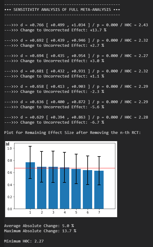
Ich habe auch eine Sensitivity-Analyse hinzugefügt, ein Standard bei Meta-Analysen. Die Meta-Analyse wird wiederholt nachgerechnet, jeweils unter Entfernung eines einzigen Experiments. Dies erlaubt zu sehen, wie stark ein bestimmtes Experiment das Gesamtergebnis beeinflusst. Die Sensitivity-Analyse erfolgt einmal für die gesamte Meta-Analyse (alle RCTs) und einmal für die auf die Top k RCTs beschränkte Analyse, letztere auch wieder mit einem verschobenem statt neuberechnetem 95 % KI.
Update 25. März 2021:
Optional kann man jetzt über die Variable year das Erscheinungsjahr der jeweiligen RCTs eingeben. Es folgt dann eine Visualisierung der Veröffentlichungen mit der Zeit und Test auf Abhängigkeit der gefundenen Effektstärken von Erscheinungsjahr. Letzterer Test ist häufig in Meta-Analysen zu finden. Für eine leere Liste year = [ ] wird dieser Abschnitt übersprungen.


Optional kann man jetzt über die Variable ind_bias den RCTs Gewichte für individuellen Bias zuordnen. Bei einem Eintrag 1 in der Liste ind_bias erfolgen keine Änderungen, bei einem Eintrag > 1 wird der Standardfehler der RCT um eben jenen Faktor erhöht. Dadurch erhält dieses RCT ein geringeres Gewicht in der Meta-Analyse. Will man z.B. bei insgesamt 5 RCTs die letzten beiden eingetragenen RCTs wegen hohem Bias-Risiko schwächer gewichten, so könnte man z.B. ind_bias = [1,1,1,1.33,1.33] setzen. Für eine leere Liste ind_bias = [ ] wird keine Anpassung vorgenommen.

Neben dem Funnel-Plot wird jetzt auch der theoretische Funnel-Plot angezeigt. Er zeigt die Regressionslinien, die man bei Abwesenheit von Publikationsbias für normalverteilte Effektstärken erhält, wenn die Anzahl RCTs gegen unendlich geht.

Einführung einer Reihe von Checks, um gängige Inputfehler zu erkennen und wenn möglich zu übergehen. Ansonsten eine saubere Beendigung des Programms.

Bekannte Fehler:
Die Interpolation beim Funnel-Plot bzw. Jahresplot erzeugt manchmal die Fehlermeldung “RuntimeWarning: invalid value encountered in power kernel_value”. Bisher bin ich noch nicht dahinter gekommen, aber die Interpolation funktioniert trotzdem und das Programm läuft ohne Probleme weiter.
Der Code:
Der aktuelle Code (25. März), geschrieben in Python 3.9. Zum Ausführen benötigt man a) einen Python-kompatiblen Compiler, b) die Installation von Python und c) die Installation aller verwendeten Module (Matplotlib, Scipy, etc …)
#%%
import matplotlib.pyplot as plt
import math
import scipy.stats
import numpy as np
import pandas as pd
import statsmodels.api as sm
from prettytable import PrettyTable
import sys

# Number to restrict

k_test = 3

# specify year and individual bias, if available, otherwise leave empty
# ind_bias = 1 -> no individual bias, ind_bias > 1 -> higher individual bias

ind_bias = [1,1,1,1,1.33,1.33,1.33]

year = [2018,2018,2013,2011,2013,2018,2006]

# input modes

# 1 = pre-formatted / 2 = d, dlow, dhigh, ... / 3 = d, se, ... / 4 = d, var, ...
# 5 = pre-formatted OR / 6 = OR, ORlow, ORhigh, ...
# 7 = pre-formatted r / 8 = r, rlow, rhigh, ...

mode = 1

if mode > 0.5 and mode < 1.5:

	d = [0.43,0.60,0.61,0.66,0.80,1.19,1.43]
	dlow = [-0.01,0.03,0.10,0.00,0.31,0.53,0.71]
	dhigh = [0.86,1.17,1.12,1.31,1.30,1.84,2.15]

if mode > 1.5 and mode < 2.5:

	l = [-0.82,-1.55,-0.09,-0.94,-1.59,-0.29,-0.65,-1.24,-0.06,-0.93,-1.45,-0.41,-0.85,-1.29,-0.41,-0.90,-1.45,-0.35,-1.13,-1.72,-0.54,-1.07,-1.51,-0.63,-0.93,-1.48,-0.38,-0.61,-1.23,0.01]

	d = []
	dlow = []
	dhigh = []

	i = 0
	while i < len(l):
		d.append(l[i])
		i += 1
		dlow.append(l[i])
		i += 1
		dhigh.append(l[i])
		i += 1

if mode > 2.5 and mode < 3.5:

	lse = [-1.39,0.34,-0.35,0.37,-1.06,0.51,-1.76,0.44,-0.86,0.28,-0.59,0.29]
	d = []
	dlow = []
	dhigh = []
	i = 0
	while i < len(lse):
		d.append(lse[i])
		davg = lse[i]
		i += 1
		low = davg-1.96*lse[i]
		dlow.append(low)
		high = davg+1.96*lse[i]
		dhigh.append(high)
		i += 1

	dlow_new = [round(x, 3) for x in dlow]
	dhigh_new = [round(x, 3) for x in dhigh]

if mode > 3.5 and mode < 4.5:

	lv = [0.1, 0.06, 0.8, 0.01, -0.2, 0.04]

	lse = []
	i = 0
	while i < len(lv):
		lse.append(lv[i])
		i += 1
		se = math.sqrt(lv[i])
		lse.append(se)
		i += 1

	d =[]
	dlow =[]
	dhigh = []
	i = 0
	while i < len(lse):
		d.append(lse[i])
		davg = lse[i]
		i += 1
		low = davg-1.96*lse[i]
		dlow.append(low)
		high = davg+1.96*lse[i]
		dhigh.append(high)
		i += 1

	lse_new = [round(x, 3) for x in lse]
	dlow_new = [round(x, 3) for x in dlow]
	dhigh_new = [round(x, 3) for x in dhigh]

if mode > 4.5 and mode < 5.5:

	OR = [1.22, 1.65, 1.82]
	ORlow = [0.93, 1.02, 1.33]
	ORhigh = [1.92, 2.11, 2.67]

	d = []
	i = 0
	while i < len(OR):
		d_temp = math.log(OR[i])*0.5513
		d.append(d_temp)
		i += 1

	dlow = []
	i = 0
	while i < len(OR):
		dlow_temp = math.log(ORlow[i])*0.5513
		dlow.append(dlow_temp)
		i += 1

	dhigh = []
	i = 0
	while i < len(OR):
		dhigh_temp = math.log(ORhigh[i])*0.5513
		dhigh.append(dhigh_temp)
		i += 1

if mode > 5.5 and mode < 6.5:

	ORl = [1.20,0.40,3.30,0.99,0.80,1.22,0.93,0.78,1.19,1.08,0.63,1.85,0.44,0.16,1.24,2.61,1.10,6.17,1.00,0.76,1.32,0.32,0.16,0.62,1.06,0.51,2.20,0.89,0.23,3.47,1.05,0.77,1.33,0.47,0.28,0.79,1.12,0.98,1.30,0.93,0.79,1.11]

	d = []
	dlow = []
	dhigh = []

	i = 0
	while i < len(ORl):
		temp = math.log(ORl[i])*0.5513
		d.append(temp)
		i += 1
		temp = math.log(ORl[i])*0.5513
		dlow.append(temp)
		i += 1
		temp = math.log(ORl[i])*0.5513
		dhigh.append(temp)
		i += 1

if mode > 6.5 and mode < 7.5:

	r = [0.55,0.35,0.38]
	rlow = [0.22,0.16,0.12]
	rhigh = [0.72,0.58,0.67]

	d = []
	i = 0
	while i < len(r):
		d_temp = 2*r[i]/math.sqrt(1-r[i]**2)
		d.append(d_temp)
		i += 1

	dlow = []
	i = 0
	while i < len(r):
		dlow_temp = 2*rlow[i]/math.sqrt(1-rlow[i]**2)
		dlow.append(dlow_temp)
		i += 1

	dhigh = []
	i = 0
	while i < len(r):
		dhigh_temp = 2*rhigh[i]/math.sqrt(1-rhigh[i]**2)
		dhigh.append(dhigh_temp)
		i += 1

if mode > 7.5 and mode < 8.5:

	rl = [0.55,0.22,0.72,0.35,0.16,0.58,0.38,0.12,0.67]

	d = []
	dlow = []
	dhigh = []

	i = 0
	while i < len(rl):
		temp = 2*rl[i]/math.sqrt(1-rl[i]**2)
		d.append(temp)
		i += 1
		temp = 2*rl[i]/math.sqrt(1-rl[i]**2)
		dlow.append(temp)
		i += 1
		temp = 2*rl[i]/math.sqrt(1-rl[i]**2)
		dhigh.append(temp)
		i += 1

print('RCT Inputs:')
print()
print('Effect Sizes d:')
print(d)
print()
print('Lower Limits of 95 % CI:')
print(dlow)
print()
print('Upper Limits of 95 % CI:')
print(dhigh)
print()
print()


# Fixed-Effects Mode: 1 = activated, 0 = deactivated
fixed_mode = 0


# k_test check to prevent error
if k_test > len(d):
	k_test = len(d)
	print('+++ Number of RCTs for restricted analysis greater than number of RCTs')
	print('+++ Number of RCTs for restricted analysis set to number of RCTs')
	print()
	print()

# k_test check to prevent error
if k_test < 1:
	k_test = 3
	print('+++ Number of RCTs for restricted analysis smaller than one')
	print('+++ Number of RCTs for restricted analysis set to three')
	print()
	print()

# ind_bias check to prevent error
if len(ind_bias) > len(d) or len(ind_bias) < len(d):
	ind_bias = []
	print('+++ Specified bias list not equal in size to effect size list')
	print('+++ Specified bias list emptied')
	print()
	print()

# year check to prevent error
if len(year) > len(d) or len(year) < len(d):
	year = []
	print('+++ Year list not equal in size to effect size list')
	print('+++ Year list emptied')
	print()
	print()

# lower limit check to prevent error
if len(dlow) > len(d) or len(dlow) < len(d):
	print('+++ Lower limit list not equal in size to effect size list')
	print('+++ Terminating Program')
	print()
	print()
	sys.exit()

# upper limit check to prevent error
if len(dhigh) > len(d) or len(dhigh) < len(d):
	print('+++ Upper limit list not equal in size to effect size list')
	print('+++ Terminating Program')
	print()
	print()
	sys.exit()


# adjustment for individual bias
if len(ind_bias) > 0:
	i = 0
	while i < len(d):
		se_here = (abs(dhigh[i]-dlow[i])/3.92)
		se_adj = ind_bias[i]*se_here
		dlow[i] = d[i]-1.96*se_adj
		dhigh[i] = d[i]+1.96*se_adj
		i += 1

	formatted_dlow = [ round(elem, 2) for elem in dlow ]
	formatted_dhigh = [ round(elem, 2) for elem in dhigh ]

	print('Individual Bias Adjusted RCT Results:')
	print()
	print('Effect Sizes d:')
	print(d)
	print()
	print('Lower Limits of 95 % CI:')
	print(formatted_dlow)
	print()
	print('Upper Limits of 95 % CI:')
	print(formatted_dhigh)
	print()
	print()


print('------------------------------------')
print(u'\u2022'u'\u2022'u'\u2022'' RANDOM-EFFECTS META-ANALYSIS 'u'\u2022'u'\u2022'u'\u2022')
print('------------------------------------')
print()

def w(x, y):
	w = 1/((abs(x-y)/3.92)**2)
	return w

wsum = 0
i = 0
while i < len(d):
	wsum = wsum + w(dlow[i], dhigh[i])
	i += 1

q1sum = 0
i = 0
while i < len(d):
	q1sum = q1sum + w(dlow[i], dhigh[i])*d[i]**2
	i += 1

q2sum = 0
i = 0
while i < len(d):
	q2sum = q2sum + w(dlow[i], dhigh[i])*d[i]
	i += 1

Q = q1sum - (q2sum**2)/wsum

c1sum = 0
i = 0
while i < len(d):
	c1sum = c1sum + w(dlow[i], dhigh[i])**2
	i += 1

C = wsum - c1sum/wsum

df = len(d) - 1


tau_squared_prelim = (Q-df)/C

if tau_squared_prelim < 0:
	tau_squared = 0
else:
	tau_squared = tau_squared_prelim


if fixed_mode > 0:
	tau_squared = 0


I_squared_prelim = 100*(Q-df)/Q

if I_squared_prelim < 0:
	I_squared = 0
else:
	I_squared = I_squared_prelim


if fixed_mode > 0:
	I_squared = 0
	Q = 0
	print('(Forcing Fixed-Effects Analysis)')
	print()

# General Information


print('Cochranes Q:', "%.2f" % Q)
print('Heterogeneity I_Squared:', "%.2f" % I_squared, '%')
print('Tau_Squared:', "%.2f" % tau_squared)
print()

print('Histogram of Effect Sizes:')
print()
plt.hist(d, density=False, bins=len(d), ec='black')
plt.ylabel('Count')
plt.xlabel('Effect Size')
plt.show()
print()

v = 1/wsum
n_total = 4/v
n_avg = n_total/len(d)


# random-effects meta-analysis

def g(x, y):
	g = 1/((abs(x-y)/3.92)**2+tau_squared)
	return g

gsum = 0
i = 0
while i < len(d):
	gsum = gsum + g(dlow[i], dhigh[i])
	i += 1

v = 1/gsum
se = math.sqrt(v)


print('RCT Weights and Imputed Sample Size:')
print()

t1 = PrettyTable(['Effect Size', 'Standard Error', 'Weight Share (%)', 'Sample Size'])

nhisto = []
i = 0
while i < len(d):

	gprint = g(dlow[i], dhigh[i])
	gshare = 100*gprint/gsum

	wprint = w(dlow[i], dhigh[i])
	vprint = 1/wprint
	nprint = round(4/vprint,0)
	nhisto.append(nprint)

	dprint = d[i]
	seprint = abs(dlow[i]-dhigh[i])/3.92

	t1.add_row(["%+.2f" % dprint,"%.2f" % seprint,"%.1f" % gshare,"%.0f" % nprint])

	i += 1


print(t1)
print()
print('Average Imputed Sample Size:', "%.0f" % n_avg)
print('Total Imputed Sample Size:', "%.0f" % n_total)

print()
print('Histogram of Sample Sizes:')
print()
plt.hist(nhisto, density=False, bins=len(nhisto),ec='black')
plt.ylabel('Count')
plt.xlabel('Sample Size')
plt.show()

print()
print('Variance of Weighted Effect:', "%.3f" % v)
print('Standard Error of Weighted Effect:', "%.3f" % se)
print()

# calculation of final results

dsum = 0
i = 0
while i < len(d):
	dsum = dsum + g(dlow[i], dhigh[i])*d[i]
	i += 1

davg = dsum/gsum

dlower = davg - 1.96*se
dupper = davg + 1.96*se

z = abs(davg/se)
p = scipy.stats.norm.sf(z)
c = abs(davg/(1.96*se)*0.85)


print('Weighted Effect with 95 % CI and One-Tailed p-Value:')
print()
print('--->>> d =', "%+.3f" % davg, '[', "%+.3f" % dlower, ',', "%+.3f" % dupper, '] / p =', "%.3f" % p, '/ H0C =',"%.2f" % c)
print()

OR = math.exp(davg*1.8138)
ORlower = math.exp(dlower*1.8138)
ORupper = math.exp(dupper*1.8138)

print('--->>> OR =', "%.3f" % OR, '[', "%.3f" % ORlower, ',', "%.3f" % ORupper, '] and p =', "%.3f" % p, '/ H0C =',"%.2f" % c)
print()

r = davg/math.sqrt(davg**2+4)
rlower = dlower/math.sqrt(dlower**2+4)
rupper = dupper/math.sqrt(dupper**2+4)

print('--->>> r =', "%+.3f" % r, '[', "%+.3f" % rlower, ',', "%+.3f" % rupper, '] and p =', "%.3f" % p, '/ H0C =',"%.2f" % c)
print()


# ------ Random-Effects Meta-Analysis Restricted to Largest RCTs ------


davg_uncorrected = davg
dlower_uncorrected = dlower
dupper_uncorrected = dupper
se_uncorrected = se
print()
print()

se_critical = 0.12

print('-----------------------------------------------------------')
print(u'\u2022'u'\u2022'u'\u2022'' RANDOM-EFFECTS META-ANALYSIS RESTRICTED TO TOP RCTs 'u'\u2022'u'\u2022'u'\u2022')
print('-----------------------------------------------------------')
print()

# ordered list creation

dtemp = list(d)
dlowtemp = list(dlow)
dhightemp = list(dhigh)

sort = []
sortlow = []
sorthigh = []

u = 1
while u < (k_test+1):

	se_min = 100
	i_min = 0

	i = 0
	while i < len(dtemp):
		se_test = abs(dhightemp[i]-dlowtemp[i])/3.92
		if se_test < se_min:
			i_min = i
			se_min = se_test
		i += 1

	sort.append(dtemp[i_min])
	sortlow.append(dlowtemp[i_min])
	sorthigh.append(dhightemp[i_min])

	dtemp.pop(i_min)
	dlowtemp.pop(i_min)
	dhightemp.pop(i_min)

	u +=1

print('Top RCTs Effect Size, SE and Imputed Sample Size:')
print()

t2 = PrettyTable(['Effect Size', 'Standard Error', 'Weight Share (%)', 'Sample Size'])

gsum = 0
i = 0
while i < k_test:
	gsum = gsum + g(sortlow[i], sorthigh[i])
	i += 1

i = 0
while i < k_test:

	se_test = abs(sorthigh[i]-sortlow[i])/3.92

	gprint = g(sortlow[i], sorthigh[i])
	gshare = 100*gprint/gsum

	wprint = w(sortlow[i], sorthigh[i])
	vprint = 1/wprint
	nprint = 4/vprint

	t2.add_row(["%+.2f" % sort[i], "%.2f" % se_test, "%.1f" % gshare, "%.0f" % nprint])

	i += 1

print(t2)
print()

d_original = list(d)
dlow_original = list(dlow)
dhigh_original = list(dhigh)

d = list(sort)
dlow = list(sortlow)
dhigh = list(sorthigh)

# Bias Testing

v = 1/gsum
se = math.sqrt(v)

dsum = 0
i = 0
while i < k_test:
	dsum = dsum + g(dlow[i], dhigh[i])*d[i]
	i += 1

davg = dsum/gsum

d_test = davg

dlower = davg - 1.96*se_uncorrected
dupper = davg + 1.96*se_uncorrected

z = abs(davg/se_uncorrected)
p = scipy.stats.norm.sf(z)

c = abs(davg/(1.96*se_uncorrected)*0.85)

print('Top Analysis with Shifted 95 % CI:')
print()
print('--->>> d =', "%+.3f" % davg, '[', "%+.3f" % dlower, ',', "%+.3f" % dupper, '] and p =', "%.3f" % p, '/ H0C =',"%.2f" % c)
print()

OR = math.exp(davg*1.8138)
ORlower = math.exp(dlower*1.8138)
ORupper = math.exp(dupper*1.8138)

print('--->>> OR =', "%.3f" % OR, '[', "%.3f" % ORlower, ',', "%.3f" % ORupper, '] and p =', "%.3f" % p, '/ H0C =',"%.2f" % c)
print()

r = davg/math.sqrt(davg**2+4)
rlower = dlower/math.sqrt(dlower**2+4)
rupper = dupper/math.sqrt(dupper**2+4)

print('--->>> r =', "%+.3f" % r, '[', "%+.3f" % rlower, ',', "%+.3f" % rupper, '] and p =', "%.3f" % p, '/ H0C =',"%.2f" % c)
print()

z_bias = abs((davg_uncorrected-davg)/se_critical)
p_bias = scipy.stats.norm.sf(z_bias)

print()
print('Difference to Calculated Effect: d =', "%.3f" % davg_uncorrected, '/ Z =', "%.3f" % z_bias, '/ p =', "%.3f" % p_bias)

davg_corrected = davg

print()
if p_bias >= 0.1:
	print('--->>> Influence of Publication Bias on Effect Size is NOT SIGNIFICANT')
if p_bias < 0.1 and p_bias >= 0.05:
	print('--->>> Influence of Publication Bias on Effect Size APPROACHES SIGNIFICANCE')
if p_bias < 0.05 and p_bias >= 0.01:
	print('--->>> Influence of Publication Bias on Effect Size is SIGNIFICANT AT p < 0.05')
if p_bias < 0.01 and p_bias >= 0.001:
	print('--->>> Influence of Publication Bias on Effect Size is SIGNIFICANT AT p < 0.01')
if p_bias < 0.001:
	print('--->>> Influence of Publication Bias on Effect Size is SIGNIFICANT AT p < 0.001')

print()
if c >= 1.1:
	print('--->>> Influence of Publication Bias on H0 Rejection is NOT CRITICAL')
if c < 1.1 and c >= 1.0:
	print('--->>> Influence of Publication Bias on H0 Rejection APPROACHES CRITICALITY')
if c < 1.0 and c >= 0.9:
	print('--->>> Influence of Publication Bias on H0 Rejection is CRITICAL')
if c < 0.9 and c >= 0.8:
	print('--->>> Influence of Publication Bias on H0 Rejection is HIGHLY CRITICAL')
if c < 0.8:
	print('--->>> Influence of Publication Bias on H0 Rejection is SEVERE')


print()
means = [davg_uncorrected, davg]

ci = [(dlower_uncorrected, dupper_uncorrected), (dlower, dupper)]

y_r = [means[i] - ci[i][1] for i in range(len(ci))]
plt.bar(range(len(means)), means, yerr=y_r, align='center', error_kw=dict(lw=2, capsize=5, capthick=2))
plt.xticks(range(len(means)), ['Original Effect','Corrected Effect'])
x = np.linspace(-0.5, len(means)-0.5)
y = 0*x
plt.plot(x, y, 'black', linewidth=0.5)
plt.show()


d = list(d_original)
dlow = list(dlow_original)
dhigh = list(dhigh_original)

print()
print()
print()
print('------------------------------------------------------------------------')
print(u'\u2022'u'\u2022'u'\u2022'' FUNNEL PLOT (D-SE) ANALYSIS CENTERED ON TOP ANALYSIS EFFECT SIZE 'u'\u2022'u'\u2022'u'\u2022')
print('------------------------------------------------------------------------')
print()

j = 0
epos = []
xpos = []
while j < len(d):
	if d[j]-d_test >= 0:
		epos.append(d[j]-d_test)
		xpos.append(abs(dhigh[j]-dlow[j])/3.92)
	j += 1

if len(epos) > 0:

	t3 = PrettyTable(['Standard Error', 'Centered Effect Size'])

	j = 0
	while j < len(epos):
		t3.add_row(["%+.2f" % xpos[j], "%+.2f" % epos[j]])
		j += 1

	print(t3)

	xpos_max = 0
	j = 0
	while j < len(epos):
		if xpos[j] > xpos_max:
			xpos_max = xpos[j]
		j += 1

	productsum = 0
	xsquaresum = 0
	j = 0
	while j < len(epos):
		productsum = productsum + xpos[j]*epos[j]
		xsquaresum = xsquaresum + xpos[j]**2
		j += 1

	slope_pos = productsum/xsquaresum

	print()
	print('Above Effect Funnel Plot:')
	print()

	plt.scatter(xpos, epos)
	plt.title("Above Effect Funnel Plot")
	plt.xlabel("Standard Error")
	plt.ylabel("Centered Effect Size")
	plt.xlim(0, xpos_max+0.05)
	x = np.linspace(0, xpos_max+0.05)
	y = slope_pos*x
	plt.plot(x, y)
	plt.show()

	print()
	print('---> Above Test Effect Zero Intercept SLOPE: ' "%+.3f" % slope_pos)
	print()
	print()

else:

	print()
	print('UNABLE TO CALCULATE Above Test Effect Regression Line')
	print()

j = 0
eneg = []
xneg = []
while j < len(d):
	if d[j]-d_test <= 0:
		eneg.append(d[j]-d_test)
		xneg.append(abs(dhigh[j]-dlow[j])/3.92)
	j += 1

if len(eneg) > 0:

	t4 = PrettyTable(['Standard Error', 'Centered Effect Size'])

	j = 0
	while j < len(eneg):
		t4.add_row(["%+.2f" % xneg[j], "%+.2f" % eneg[j]])
		j += 1

	print(t4)

	productsum = 0
	xsquaresum = 0
	j = 0
	while j < len(eneg):
		productsum = productsum + xneg[j]*eneg[j]
		xsquaresum = xsquaresum + xneg[j]**2
		j += 1

	slope_neg = productsum/xsquaresum

	xneg_max = 0
	j = 0
	while j < len(eneg):
		if xneg[j] > xneg_max:
			xneg_max = xneg[j]
		j += 1

	print()
	print('Below Effect Funnel Plot:')
	print()

	plt.scatter(xneg, eneg)
	plt.title("Above Effect Funnel Plot")
	plt.xlabel("Standard Error")
	plt.ylabel("Centered Effect Size")
	plt.xlim(0, xneg_max+0.05)
	x = np.linspace(0, xneg_max+0.05)
	y = slope_neg*x
	plt.plot(x, y)
	plt.show()

	print()
	print('---> Below Test Effect Zero Intercept SLOPE: ' "%+.3f" % slope_neg)
	print()

	print()
	print('Complete Funnel Plot:')
	print()

	x = xneg+xpos
	e = eneg+epos

	if xneg_max > xpos_max:
		xmax = xneg_max
	else:
		xmax = xpos_max

	plt.scatter(x, e)
	plt.title("Funnel Plot")
	plt.xlabel("Standard Error")
	plt.ylabel("Centered Effect Size")
	plt.xlim(0, xmax+0.05)
	x = np.linspace(0, xmax+0.05)
	y = slope_pos*x
	plt.plot(x, y)
	x = np.linspace(0, xmax+0.05)
	y = slope_neg*x
	plt.plot(x, y)
	x = np.linspace(0, xmax+0.05)
	y = 0*x
	plt.plot(x, y,'black', linewidth=0.5)
	plt.show()

	print()

	x = xneg+xpos
	e = eneg+epos

	print()
	print('Comparison to Theoretical Funnel Plot Regression Lines:')
	print()

	plt.scatter(x, e)
	plt.title("Theoretical Funnel Plot")
	plt.xlabel("Standard Error")
	plt.ylabel("Centered Effect Size")
	plt.xlim(0, xmax+0.05)
	x = np.linspace(0, xmax+0.05)
	y = 0.8*x
	plt.plot(x, y)
	x = np.linspace(0, xmax+0.05)
	y = -0.8*x
	plt.plot(x, y)
	x = np.linspace(0, xmax+0.05)
	y = 0*x
	plt.plot(x, y, 'black', linewidth=0.5)
	plt.show()


	from statsmodels.nonparametric.kernel_regression import KernelReg

	X = xneg+xpos
	Y = eneg+epos

	# Combine lists into list of tuples
	points = zip(X, Y)

	# Sort list of tuples by x-value
	points = sorted(points, key=lambda point: point[0])

	# Split list of tuples into two list of x values any y values
	X, Y = zip(*points)

	print()
	print()
	print('Funnel Plot Interpolation:')
	print()

	kr = KernelReg(Y,X,'o')
	y_pred, y_std = kr.fit(X)
	plt.xlim(0, xmax+0.05)
	plt.scatter(X,Y, s = 20)
	plt.title("Funnel Plot")
	plt.xlabel("Standard Error")
	plt.ylabel("Centered Effect Size")
	x = np.linspace(0, xmax+0.05)
	y = 0*x
	plt.plot(x, y, 'black', linewidth=0.5)
	plt.plot(X, y_pred, color = 'orange')
	plt.show()

	print()
	print('R_Squared =',"%.2f" % kr.r_squared())
	print()

else:

	print()
	print('UNABLE TO CALCULATE Below Test Effect Regression Line')
	print()

if len(epos) > 0 and len(eneg) > 0:

	if davg_uncorrected > 0:
		if abs(slope_neg) > slope_pos:
			prob = 100
		else:
			prob = 100*(0.3*math.exp(-abs(slope_neg))+abs(slope_neg))/(0.3*math.exp(-abs(slope_pos))+slope_pos)
	else:
		if slope_pos > abs(slope_neg):
			prob = 100
		else:
			prob = 100*(0.3*math.exp(-abs(slope_pos))+slope_pos)/(0.3*math.exp(-abs(slope_neg))+abs(slope_neg))

	print()

	slope_diff = slope_pos-abs(slope_neg)

	print(u'\u2022'' TEST FOR FUNNEL PLOT ASYMMETRIES:')
	print()
	print()

	print('Slopes: ' "%.3f" % slope_pos, 'Above Effect versus', "%.3f" % slope_neg, 'Below Effect')
	print('Slope Difference: ' "%.3f" % slope_diff)
	print()
	print('---> Estimated Probability of Publishing Undesired Result:', "%.0f" % prob, '%')
	if prob >= 83:
		print('---> Slope Asymmetry Implies INSIGNIFICANT Publication Bias')
	if prob < 83 and prob >= 65:
		print('---> Slope Asymmetry Implies SLIGHT Publication Bias')
	if prob < 65 and prob >= 48:
		print('---> Slope Asymmetry Implies MODERATE Publication Bias')
	if prob < 48 and prob >= 30:
		print('---> Slope Asymmetry Implies STRONG Publication Bias')
	if prob < 30:
		print('---> Slope Asymmetry Implies SEVERE Publication Bias')
	print()

else:

	print()
	print('UNABLE TO CALCULATE Slope Difference')
	print()

if len(epos) > 0 and len(eneg) > 0:

	ipos = len(xpos)
	ineg = len(xneg)
	iref = max(ipos,ineg)

	n_diff_raw = 100*(ipos-ineg)/iref
	n_diff = 100*(ipos-ineg)/(iref+2)

	print()
	print('RCT Counts: ' "%.0f" % ipos, 'Above Effect versus', "%.0f" % ineg, 'Below Effect')
	print('RCT Count Asymmetry Raw: ' "%+.0f" % n_diff_raw, '%')
	print('RCT Count Asymmetry Corrected: ' "%+.0f" % n_diff, '%')

	if davg_uncorrected > 0:
		if n_diff < 0:
			prob1 = 100
		else:
			prob1 = 100-n_diff
	else:
		if n_diff > 0:
			prob1 = 100
		else:
			prob1 = 100-abs(n_diff)

	print()
	print('---> Estimated Probability of Publishing Undesired Result:', "%.0f" % prob1, '%')
	if prob1 >= 83:
		print('---> RCT Count Asymmetry Implies INSIGNIFICANT Publication Bias')
	if prob1 < 83 and prob1 >= 65:
		print('---> RCT Count Asymmetry Implies SLIGHT Publication Bias')
	if prob1 < 65 and prob1 >= 48:
		print('---> RCT Count Asymmetry Implies MODERATE Publication Bias')
	if prob1 < 48 and prob1 >= 30:
		print('---> RCT Count Asymmetry Implies STRONG Publication Bias')
	if prob1 < 30:
		print('---> RCT Count Asymmetry Implies SEVERE Publication Bias')
	print()


	outlierpos = 0
	j = 0
	while j < len(epos):
		if epos[j] > 0.5:
			outlierpos = outlierpos + 1
		j += 1

	outlierneg = 0
	j = 0
	while j < len(eneg):
		if eneg[j] < -0.5:
			outlierneg = outlierneg + 1
		j += 1

	iref = max(outlierpos,outlierneg)

	if iref <= 0: iref = 1

	outlier_diff_raw = 100*(outlierpos-outlierneg)/iref
	outlier_diff = 100*(outlierpos-outlierneg)/(iref+1)

	print()
	print('RCT Outlier Counts: ' "%.0f" % outlierpos, 'Above Effect versus', "%.0f" % outlierneg, 'Below Effect')
	print('Outlier Asymmetry Raw: ' "%+.0f" % outlier_diff_raw, '%')
	print('Outlier Asymmetry Corrected: ' "%+.0f" % outlier_diff, '%')

	if davg_uncorrected > 0:
		if outlier_diff < 0:
			prob2 = 100
		else:
			prob2 = 100-outlier_diff
	else:
		if outlier_diff > 0:
			prob2 = 100
		else:
			prob2 = 100-abs(outlier_diff)

	print()
	print('---> Estimated Probability of Publishing Undesired Result:', "%.0f" % prob2, '%')
	if prob2 >= 83:
		print('---> Outlier Asymmetry Implies INSIGNIFICANT Publication Bias')
	if prob2 < 83 and prob2 >= 65:
		print('---> Outlier Asymmetry Implies SLIGHT Publication Bias')
	if prob2 < 65 and prob2 >= 48:
		print('---> Outlier Asymmetry Implies MODERATE Publication Bias')
	if prob2 < 48 and prob2 >= 30:
		print('---> Outlier Asymmetry Implies STRONG Publication Bias')
	if prob2 < 30:
		print('---> Outlier Asymmetry Implies SEVERE Publication Bias')
	print()


	distance_pos = 0
	j = 0
	while j < len(epos):
		distance_pos = distance_pos+epos[j]
		j += 1

	distance_neg = 0
	j = 0
	while j < len(eneg):
		distance_neg = distance_neg+eneg[j]
		j += 1

	distance_ref = max(distance_pos,abs(distance_neg))

	distance_diff_raw = 100*(distance_pos+distance_neg)/distance_ref
	distance_diff = 100*(distance_pos+distance_neg)/(distance_ref+0.4)

	print()
	print('Effect Distance Sums: ' "%.2f" % distance_pos, 'Above Effect versus', "%.2f" % distance_neg, 'Below Effect')
	print('Effect Distance Sum Asymmetry Raw: ' "%+.0f" % distance_diff_raw, '%')
	print('Effect Distance Sum Asymmetry Corrected: ' "%+.0f" % distance_diff, '%')

	if davg_uncorrected > 0:
		if distance_diff < 0:
			prob3 = 100
		else:
			prob3 = 100-abs(distance_diff)
	else:
		if distance_diff > 0:
			prob3 = 100
		else:
			prob3 = 100-abs(distance_diff)

	print()
	print('---> Estimated Probability of Publishing Undesired Result:', "%.0f" % prob3, '%')
	if prob3 >= 83:
		print('---> Effect Distance Sum Asymmetry Implies INSIGNIFICANT Publication Bias')
	if prob3 < 83 and prob3 >= 65:
		print('---> Effect Distance Sum Asymmetry Implies SLIGHT Publication Bias')
	if prob3 < 65 and prob3 >= 48:
		print('---> Effect Distance Sum Asymmetry Implies MODERATE Publication Bias')
	if prob3 < 48 and prob3 >= 30:
		print('---> Effect Distance Sum Asymmetry Implies STRONG Publication Bias')
	if prob3 < 30:
		print('---> Effect Distance Sum Asymmetry Implies SEVERE Publication Bias')
	print()


	epos_max = 0
	j = 0
	while j < len(epos):
		if epos[j] > epos_max:
			epos_max = epos[j]
		j += 1

	eneg_max = 0
	j = 0
	while j < len(eneg):
		if eneg[j] < eneg_max:
			eneg_max = eneg[j]
		j += 1

	maxeffect_ref = max(epos_max,abs(eneg_max))

	maxeffect_diff_raw = 100*(epos_max+eneg_max)/maxeffect_ref
	maxeffect_diff = 100*(epos_max+eneg_max)/(maxeffect_ref+0.1)

	print()
	print('Effect Ranges: ' "%.2f" % epos_max, 'Above Effect versus', "%.2f" % eneg_max, 'Below Effect')
	print('Effect Range Asymmetry Raw: ' "%+.0f" % maxeffect_diff_raw, '%')
	print('Effect Range Asymmetry Corrected: ' "%+.0f" % maxeffect_diff, '%')

	if davg_uncorrected > 0:
		if maxeffect_diff < 0:
			prob4 = 100
		else:
			prob4 = 100-abs(maxeffect_diff)
	else:
		if maxeffect_diff > 0:
			prob4 = 100
		else:
			prob4 = 100-abs(maxeffect_diff)

	print()
	print('---> Estimated Probability of Publishing Undesired Result:', "%.0f" % prob4, '%')
	if prob4 >= 83:
		print('---> Effect Range Asymmetry Implies INSIGNIFICANT Publication Bias')
	if prob4 < 83 and prob4 >= 65:
		print('---> Effect Range Asymmetry Implies SLIGHT Publication Bias')
	if prob4 < 65 and prob4 >= 48:
		print('---> Effect Range Asymmetry Implies MODERATE Publication Bias')
	if prob4 < 48 and prob4 >= 30:
		print('---> Effect Range Asymmetry Implies STRONG Publication Bias')
	if prob4 < 30:
		print('---> Effect Range Asymmetry Implies SEVERE Publication Bias')
	print()


	gw = (100/prob)**1.33
	gw1 = (100/prob1)**1.33
	gw2 = (100/prob2)**1.33
	gw3 = (100/prob3)**1.33
	gw4 = (100/prob4)**1.33

	gwsum = gw + gw1 + gw2 + gw3 + gw4

	prob_mean = (gw*prob+gw1*prob1+gw2*prob2+gw3*prob3+gw4*prob4)/gwsum

	ugw = (100/prob)
	ugw1 = (100/prob1)
	ugw2 = (100/prob2)
	ugw3 = (100/prob3)
	ugw4 = (100/prob4)

	ugwsum = ugw + ugw1 + ugw2 + ugw3 + ugw4

	uvar = 1/ugwsum
	use = 100*math.sqrt(uvar)

	prob_lower = prob_mean - 0.75*use
	prob_upper = prob_mean + 0.75*use

	print()
	print(u'\u2022'' COMBINED FUNNEL PLOT ANALYSIS:')
	print()
	print('--->>> Estimated Probability of Publishing Undesired Result:', "%.0f" % prob_mean, '% [', "%.0f" % prob_lower, '% ,', "%.0f" % prob_upper, '% ]')
	if prob_mean >= 83:
		print('--->>> Funnel Plot Analysis Implies INSIGNIFICANT Publication Bias')
	if prob_mean < 83 and prob_mean >= 65:
		print('--->>> Funnel Plot Analysis Implies SLIGHT Publication Bias')
	if prob_mean < 65 and prob_mean >= 48:
		print('--->>> Funnel Plot Analysis Implies MODERATE Publication Bias')
	if prob_mean < 48 and prob_mean >= 30:
		print('--->>> Funnel Plot Analysis Implies STRONG Publication Bias')
	if prob_mean < 30:
		print('--->>> Funnel Plot Analysis Implies SEVERE Publication Bias')

else:

	print()
	print('UNABLE TO CALCULATE Asymmetries')
	print()

print()
print('Imputed Probabilities of Publishing Undesired Results:')
print()
means = [prob, prob1, prob2, prob3, prob4, prob_mean]

ci = [(prob,prob),(prob1,prob1),(prob2,prob2),(prob3,prob3),(prob4,prob4), (prob_lower, prob_upper)]

y_r = [means[i] - ci[i][1] for i in range(len(ci))]
plt.bar(range(len(means)), means, yerr=y_r, align='center', error_kw=dict(lw=2, capsize=5, capthick=2))
plt.xticks(range(len(means)), ['Slopes','Counts', 'Outliers', 'Distances', 'Ranges', 'Combined'])
plt.show()


print()
print()
print()
print('--------------------------------------------------')
print(u'\u2022'u'\u2022'u'\u2022'' SENSITIVITY ANALYSIS OF FULL META-ANALYSIS 'u'\u2022'u'\u2022'u'\u2022')
print('--------------------------------------------------')
print()

dremain = []
dlowerremain = []
dupperremain = []

changesum = 0
changemax = 0
minhoc = 100

n = 0
while n < len(d_original):

	d = list(d_original)
	dlow = list(dlow_original)
	dhigh = list(dhigh_original)

	del d[n]
	del dlow[n]
	del dhigh[n]

	wsum = 0
	i = 0
	while i < len(d):
		wsum = wsum + w(dlow[i], dhigh[i])
		i += 1

	q1sum = 0
	i = 0
	while i < len(d):
		q1sum = q1sum + w(dlow[i], dhigh[i])*d[i]**2
		i += 1

	q2sum = 0
	i = 0
	while i < len(d):
		q2sum = q2sum + w(dlow[i], dhigh[i])*d[i]
		i += 1

	Q = q1sum - (q2sum**2)/wsum

	c1sum = 0
	i = 0
	while i < len(d):
		c1sum = c1sum + w(dlow[i], dhigh[i])**2
		i += 1

	C = wsum - c1sum/wsum

	df = len(d) - 1


	tau_squared_prelim = (Q-df)/C

	if tau_squared_prelim < 0:
		tau_squared = 0
	else:
		tau_squared = tau_squared_prelim


	if fixed_mode > 0:
		tau_squared = 0


	I_squared_prelim = 100*(Q-df)/Q

	if I_squared_prelim < 0:
		I_squared = 0
	else:
		I_squared = I_squared_prelim


	if fixed_mode > 0:
		I_squared = 0
		Q = 0

	# random-effects meta-analysis

	gsum = 0
	i = 0
	while i < len(d):
		gsum = gsum + g(dlow[i], dhigh[i])
		i += 1

	v = 1/gsum
	se = math.sqrt(v)

	# calculation of final results

	dsum = 0
	i = 0
	while i < len(d):
		dsum = dsum + g(dlow[i], dhigh[i])*d[i]
		i += 1

	davg = dsum/gsum

	dremain.append(davg)

	dlower = davg - 1.96*se
	dupper = davg + 1.96*se

	dlowerremain.append(dlower)
	dupperremain.append(dupper)

	z = abs(davg/se)
	p = scipy.stats.norm.sf(z)

	c = abs(davg/(1.96*se)*0.85)

	if c < minhoc:
		minhoc = c

	change = 100*(davg-davg_uncorrected)/davg_uncorrected
	changesum = changesum + abs(change)

	if abs(change) > changemax:
		changemax = abs(change)

	print('--->>> d =', "%+.3f" % davg, '[', "%+.3f" % dlower, ',', "%+.3f" % dupper, '] / p =', "%.3f" % p, '/ H0C =',"%.2f" % c)
	print('--->>> Change to Uncorrected Effect:', "%+.1f" % change, '%')
	print()

	n += 1

print('Plot for Remaining Effect Size after Removing the n-th RCT:')
print()


means = []
labels = []
n = 0
while n < len(dremain):
	means.append(dremain[n])
	labels.append(n+1)
	n += 1

ci = []
n = 0
while n < len(dremain):
	ci.append((dlowerremain[n],dupperremain[n]))
	n += 1

y_r = [means[i] - ci[i][1] for i in range(len(ci))]
plt.bar(range(len(means)), means, yerr=y_r, align='center', error_kw=dict(lw=2, capsize=5, capthick=2))
plt.xticks(range(len(means)), labels)
plt.axhline(y=davg_uncorrected,linewidth=1, color='red')
x = np.linspace(-1, len(dremain))
y = 0*x
plt.plot(x, y, 'black', linewidth=0.5)
plt.show()

changeavg = changesum/len(dremain)

print()
print('Average Absolute Change:', "%.1f" % changeavg, '%')
print('Maximum Absolute Change:', "%.1f" % changemax, '%')
print()
print('Minimum H0C:', "%.2f" % minhoc)


if k_test > 1:

	print()
	print()
	print()
	print('--------------------------------------------------------')
	print(u'\u2022'u'\u2022'u'\u2022'' SENSITIVITY ANALYSIS OF RESTRICTED META-ANALYSIS 'u'\u2022'u'\u2022'u'\u2022')
	print('--------------------------------------------------------')
	print()

	dremain = []
	dlowerremain = []
	dupperremain = []

	changesum = 0
	changemax = 0
	minhoc = 100

	n = 0
	while n < len(sort):

		d = list(sort)
		dlow = list(sortlow)
		dhigh = list(sorthigh)

		del d[n]
		del dlow[n]
		del dhigh[n]

		wsum = 0
		i = 0
		while i < len(d):
			wsum = wsum + w(dlow[i], dhigh[i])
			i += 1

		q1sum = 0
		i = 0
		while i < len(d):
			q1sum = q1sum + w(dlow[i], dhigh[i])*d[i]**2
			i += 1

		q2sum = 0
		i = 0
		while i < len(d):
			q2sum = q2sum + w(dlow[i], dhigh[i])*d[i]
			i += 1

		Q = q1sum - (q2sum**2)/wsum

		c1sum = 0
		i = 0
		while i < len(d):
			c1sum = c1sum + w(dlow[i], dhigh[i])**2
			i += 1

		C = wsum - c1sum/wsum

		df = len(d) - 1

		if k_test > 2:
			tau_squared_prelim = (Q-df)/C

			if tau_squared_prelim < 0:
				tau_squared = 0
			else:
				tau_squared = tau_squared_prelim
		else:
			tau_squared = 0

		if fixed_mode > 0:
			tau_squared = 0

		if k_test > 2:
			I_squared_prelim = 100*(Q-df)/Q

			if I_squared_prelim < 0:
				I_squared = 0
			else:
				I_squared = I_squared_prelim
		else:
			I_squared = 0

		if fixed_mode > 0:
			I_squared = 0
			Q = 0

		# random-effects meta-analysis

		gsum = 0
		i = 0
		while i < len(d):
			gsum = gsum + g(dlow[i], dhigh[i])
			i += 1

		v = 1/gsum
		se = math.sqrt(v)

		# calculation of final results

		dsum = 0
		i = 0
		while i < len(d):
			dsum = dsum + g(dlow[i], dhigh[i])*d[i]
			i += 1

		davg = dsum/gsum

		dremain.append(davg)

		dlower = davg - 1.96*se_uncorrected
		dupper = davg + 1.96*se_uncorrected

		dlowerremain.append(dlower)
		dupperremain.append(dupper)

		z = abs(davg/se_uncorrected)
		p = scipy.stats.norm.sf(z)

		c = abs(davg/(1.96*se_uncorrected)*0.85)

		if c < minhoc:
			minhoc = c

		change = 100*(davg-davg_corrected)/davg_corrected
		changesum = changesum + abs(change)

		if abs(change) > changemax:
			changemax = abs(change)

		print('--->>> d =', "%+.3f" % davg, '[', "%+.3f" % dlower, ',', "%+.3f" % dupper, '] / p =', "%.3f" % p, '/ H0C =',"%.2f" % c)
		print('--->>> Change to Corrected Effect:', "%+.1f" % change, '%')
		print()

		n += 1

	print('Plot for Remaining Effect Size after Removing the n-th RCT:')
	print()

	means = []
	labels = []
	n = 0
	while n < len(dremain):
		means.append(dremain[n])
		labels.append(n+1)
		n += 1

	ci = []
	n = 0
	while n < len(dremain):
		ci.append((dlowerremain[n],dupperremain[n]))
		n += 1

	y_r = [means[i] - ci[i][1] for i in range(len(ci))]
	plt.bar(range(len(means)), means, yerr=y_r, align='center', error_kw=dict(lw=2, capsize=5, capthick=2))
	plt.xticks(range(len(means)), labels)
	plt.axhline(y=davg_corrected,linewidth=1, color='red')
	x = np.linspace(-1, len(dremain))
	y = 0*x
	plt.plot(x, y, 'black', linewidth=0.5)
	plt.show()

	changeavg = changesum/len(dremain)

	print()
	print('Average Absolute Change:', "%.1f" % changeavg, '%')
	print('Maximum Absolute Change:', "%.1f" % changemax, '%')
	print()
	print('Minimum H0C:', "%.2f" % minhoc)


if len(year) > 0:

	print()
	print()
	print()
	print('---------------------------')
	print(u'\u2022'u'\u2022'u'\u2022'' TIME-SERIES OF RCTS 'u'\u2022'u'\u2022'u'\u2022')
	print('---------------------------')
	print()

	yearmin = 10000
	i = 0
	while i < len(d_original):
		if year[i] < yearmin:
			yearmin = year[i]
		i += 1

	yearmax = 0
	i = 0
	while i < len(d_original):
		if year[i] > yearmax:
			yearmax = year[i]
		i += 1

	print('Earliest RCT:', yearmin)
	print('Most Recent RCT:',yearmax)
	print()

	yearrange = yearmax-yearmin

	yearlist = []
	i = 0
	while i < yearrange+1:
		yearlist.append(yearmin+i)
		i += 1

	numberstudies = []
	i = 0
	while i < yearrange+1:
		number = year.count(yearmin+i)
		numberstudies.append(number)
		i += 1

	print('Number of RCTs Over Time:')
	print()

	fig = plt.figure()
	ax = fig.add_axes([0,0,1,1])
	ax.bar(yearlist,numberstudies)
	plt.show()

	X = year
	Y = d_original

	print()
	print('Linear Regression Test of Effect Sizes Over Time:')

	model = sm.OLS(Y,sm.add_constant(X))
	results = model.fit()
	plt.scatter(X,Y, s = 20)
	X_plot = np.linspace(yearmin-2,yearmax+2,100)
	plt.plot(X_plot, results.params[0] + X_plot*results.params[1], color = 'orange')
	print()
	plt.show()

	print()
	print('Slope =', "%+.2f" % results.params[1], '/ p =', "%.3f" % results.pvalues[1])
	print('R_Squared =',"%.2f" % results.rsquared)
	print()
	print('Interpolation of Effect Sizes Over Time:')
	print()

	from statsmodels.nonparametric.kernel_regression import KernelReg

	# Combine lists into list of tuples
	points = zip(X, Y)

	# Sort list of tuples by x-value
	points = sorted(points, key=lambda point: point[0])

	# Split list of tuples into two list of x values any y values
	X, Y = zip(*points)

	kr = KernelReg(Y,X,'o')
	y_pred, y_std = kr.fit(X)
	plt.xlim(yearmin-2, yearmax+2)
	plt.scatter(X,Y, s = 20)
	plt.plot(X, y_pred, color = 'orange')
	plt.show()

	print()
	print('R_Squared =',"%.2f" % kr.r_squared())
[…] von Walter S. Marcantoni. Ich habe die Daten dieser Meta-Analyse mal durch mein Programm Autobias gejagt, um zu sehen, wie es in diesem Fall um den Publikationsbias steht und ob sich auch nach […]
LikeLike
[…] von Walter S. Marcantoni. Ich habe die Daten dieser Meta-Analyse mal durch mein Programm Autobias gejagt, um zu sehen, wie es in diesem Fall um den Publikationsbias steht und ob sich auch nach […]
LikeLike
[…] von Walter S. Marcantoni. Ich habe die Daten dieser Meta-Analyse mal durch mein Programm Autobias gejagt, um zu sehen, wie es in diesem Fall um den Publikationsbias steht und ob sich auch nach […]
LikeLike
[…] von Walter S. Marcantoni. Ich habe die Daten dieser Meta-Analyse mal durch mein Programm Autobias gejagt, um zu sehen, wie es in diesem Fall um den Publikationsbias steht und ob sich auch nach […]
LikeLike
[…] von Walter S. Marcantoni. Ich habe die Daten dieser Meta-Analyse mal durch mein Programm Autobias gejagt, um zu sehen, wie es in diesem Fall um den Publikationsbias steht und ob sich auch nach […]
LikeLike
[…] von Walter S. Marcantoni. Ich habe die Daten dieser Meta-Analyse mal durch mein Programm Autobias gejagt, um zu sehen, wie es in diesem Fall um den Publikationsbias steht und ob sich auch nach […]
LikeLike